


Linear Regression
Or how to draw the best line through a cloud of dots
You’ve probably looked at a chart at some point and thought: «yeah, this clearly goes up.» Well, congratulations: your brain just did a linear regression by eye.
That’s exactly what Linear Regression is: finding the straight line that best sums up a cloud of dots. It’s the first thing almost everyone learns when they step into Machine Learning, which is why a lot of people brush it off as «too easy.»
Big mistake. Because this humble little line hides nearly every idea that later powers the fancier models:
- the idea of learning from data by tweaking a few numbers,
- the idea of measuring how wrong we are,
- the idea of improving that error little by little,
- and the foundation that neural networks and deep learning are built on top of.
Which is why people say something that really isn’t an exaggeration:
If you truly understand Linear Regression, you’re halfway through classic ML.
Let’s take it slow.
1. What problem does it solve?
Picture a table with two columns. In one, you write down something you know (the hours someone studied, the size of an apartment, the temperature on a given day). In the other, something you’d like to guess (the exam grade, the apartment’s price, ice cream sales).
The question is always the same:
«If I know the first column, can I predict the second?»
Linear Regression answers with the simplest solution possible: drawing a single straight line that connects the two. Once you have that line, predicting is trivial: drop in your input, see where the line lands, and there’s your prediction.
That line has just two knobs controlling it:
- one moves it up or down as a whole,
- the other tilts it more or less.
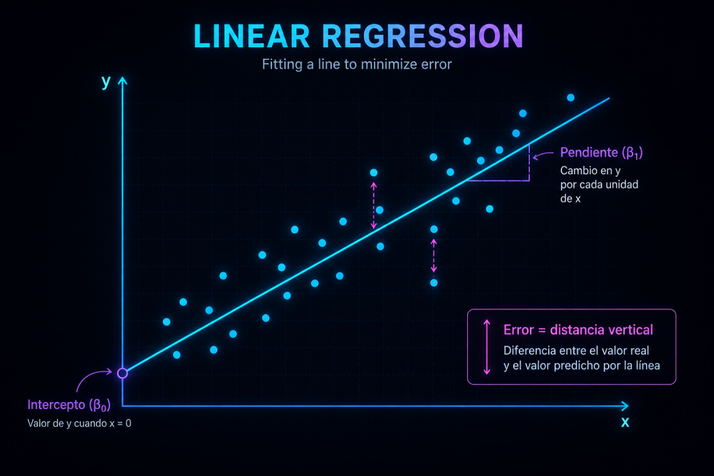
That’s it. By adjusting those two knobs you can place the line anywhere. Mathematicians call them the intercept and the slope, and they write it like this:
ŷ = β₀ + β₁·x
Don’t let the symbols scare you: β₀ is the knob that moves it up and down, β₁ is the one that tilts it, and ŷ is simply the prediction that comes out at the end. We’ll come back to them.
2. The key idea: don’t leave any dot too far away
Here’s the heart of it all, and it’s much easier to grasp with a mental image.
Picture your data as a bunch of dots scattered across a sheet of paper. Your mission is to draw a straight line that runs «between all of them.» The catch is that no line will ever pass through every dot at once: some will end up above your line and others below.
That leftover gap between a dot and the line is what we call the error: it’s how much the model got that particular dot wrong.
Regression looks for the line that keeps every dot as close as possible. But there’s a clever trick in how it measures that closeness: instead of adding up the distances as they are, it squares them.
Why the trick? For three pretty intuitive reasons:
- It makes the big misses hurt more. A dot that lands way off gets penalized heavily, so the model genuinely tries hard not to abandon anyone out in the middle of nowhere.
- It stops errors from cancelling each other out. Without squaring, one dot far above and another far below would balance out and give a false sense that «everything’s fine.»
- It makes the math cleaner, so the computer can find the best line in a tidy way.
This method of «picking the line that minimizes the squared errors» has a fancy name: Ordinary Least Squares. But the idea, as you can see, is plain common sense.
3. The slope: the model’s most useful number
Of the line’s two knobs, the slope (that β₁) is the most interesting one, because it tells you a story in plain human language:
«For every unit the input goes up, the prediction moves by this much.»
Let’s use a real-life example. Say we train the model on study data and the slope turns out to be 0.5. The translation is:
For every extra hour you study, your grade goes up half a point.
Simple and powerful. If the slope were a negative number, the story would flip: when one thing goes up, the other goes down (for example, the more screen time before bed, the fewer hours of sleep).
This is what makes Linear Regression so special compared to more «black box» models: it doesn’t just hand you a number, it explains the relationship between things. It’s a model you can actually read and understand.
4. And the other knob, the up-and-down one?
The intercept (β₀) is simply the line’s starting height: the value the model predicts when the input is zero.
Its job is to let the line sit at the right height. Without it, we’d force the line to always start from the floor (the zero point), and that almost never fits real data.
One honest warning, though: the intercept doesn’t always mean something in the real world. If your input is the size of a house, a «zero-square-meter» apartment doesn’t exist, so its prediction has no practical meaning. But the model still needs it to work properly. Think of it as an internal part of the machine: you don’t always look at it, but without it the whole thing limps.
5. How does the computer find the best line?
Okay, we know what we want: the line with the smallest possible error. But how does the machine find it? There are two ways, and both are worth knowing.
The fast lane: the magic formula.
For Linear Regression there’s a mathematical formula that spits out the perfect line in a single calculation, no trial and error. It’s like having the solved sudoku printed right next to you: direct and exact. The usual libraries (like Scikit-Learn) use it whenever they can, because it’s fast and precise.
The step-by-step lane: guess and correct.
The second way is more hands-on: the computer starts with some random line, checks how wrong it is, nudges it a little, checks again, nudges again… and keeps going until the error is as small as it gets. It’s like tuning a guitar: you turn the peg bit by bit until the string sounds right.
This second approach has a name, gradient descent, and even though it seems like the less elegant one, it’s far more important in the long run: it’s the engine behind almost all modern ML, from neural networks to deep learning.
In Part 2 we’ll look at exactly how the model measures its error.
In Part 3 we’ll take that «tuning» apart step by step.
6. Why does such an old model still matter so much?
For two reasons: because of everything it teaches you and everything it’s still used for.
As a first model, it’s a masterclass disguised as something simple. By learning it, you suddenly understand ideas that show up everywhere in the field: how a model learns from data, how you measure an error, how you improve it, how you read a result, and even how problems start when a model «memorizes the data.»
And as a real tool, it’s nowhere near a textbook relic. Right now it’s used to:
- predict sales and demand in businesses,
- set prices,
- understand what causes what in studies and analysis,
- power economic models,
- and form part of bigger prediction systems.
Which is why many call it the most underrated model in Machine Learning: so simple it gets ignored, so fundamental it’s everywhere.
In a nutshell
- Linear Regression looks for the line that keeps every dot as close as possible.
- It does this by punishing big errors more (that’s why it squares the distances).
- The slope tells you how much the prediction moves when the input changes; it’s what makes the model easy to interpret.
- The intercept sets the line at the right height.
- The computer finds that line with a direct formula or by guessing and correcting little by little.
- Understanding it well means understanding the foundation of almost all Machine Learning.