Linear Regression (Part 2)

The cost function: how the model measures its error and why it learns by minimizing

In Part 1 we covered the intuition: a straight line, two knobs (slope and intercept), and a cloud of points we want to keep as close to that line as possible.

But we left out the single most important question of all:

How does the model know whether it’s doing well or badly?

Because without a way to measure error, there’s no learning. And without learning, there’s no Machine Learning. So today we get to the heart of the model: the cost function.

---

1. The error point by point: the vertical distance

Every point in your data has two sides:

• an actual value, which we call yi​,
• and a prediction from the model, which we call y^​i​.

The difference between the two is the error for that point:

errori​=yi​−y^​i​

If the prediction falls below the real point, the error is positive; if it falls above, it’s negative. But that sign doesn’t matter yet. The only thing that matters for now is that every point contributes its own error.

---

2. The problem: errors cancel each other out

What if we just summed all the errors as they are?

∑i=1n​(yi​−y^​i​)

We’d have a huge problem: an error of +5 and another of –5 would cancel each other out, and the result would be zero. The model would think everything is perfect.

But it isn’t perfect. It’s terrible. We need a way to stop the errors from offsetting one another.

---

3. The elegant solution: squaring

Here comes the master trick. Instead of summing the errors, we sum their squares:

(yi​−y^​i​)2

Why square them? For three reasons that make a lot of sense:

1. Big errors hurt more. A miss of 10 doesn’t count «10 times more» than a miss of 1: it counts 100 times more. This forces the model to take the far-off points seriously.
2. It prevents cancellations. Any number squared is positive, so there’s no longer any way for one error to compensate for another.
3. It smooths out the math. Squaring gives us a «smooth,» differentiable function, something that will be key for the gradient descent in Part 3.

---

4. The full cost function: the MSE

If we put all the squared errors together and take the average, we get the cost function:

J(β0​,β1​)=n1​∑i=1n​(yi​−y^​i​)2

This has a name of its own:

✔️ MSE — Mean Squared Error

It’s the most widely used metric in regression, and it basically sums up in a single number how wrong the model is across all of your data at once.

---

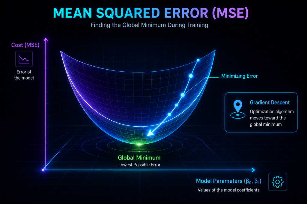
5. What does it mean to «minimize» this function?

Here’s the beautiful part. Imagine the cost function is a landscape: a smooth hill, with no weird peaks or traps.

Each point in that landscape corresponds to a specific combination of the model’s two knobs:

• β0​, the intercept,
• β1​, the slope.

And the height at each point is the error (the MSE) that combination produces. With this picture in mind, learning becomes very easy to understand:

Learning is finding the lowest point in that landscape.

And that lowest point is, quite simply, the perfect line.

---

6. Why is this landscape so special?

Because it has a wonderful property: it’s convex. In plain terms, that means it’s bowl-shaped, and therefore:

• there are no false minima,
• there are no hidden valleys to get stuck in,
• there’s only one single global minimum.

Put another way: wherever you start, if you keep walking downhill you’ll always reach the same bottom. This makes Linear Regression one of the most stable and predictable models in all of classical ML.

---

7. So how does the model walk down that hill?

Here’s where the star of Part 3 pokes its head out: ⭐ gradient descent.

The idea is very simple:

1. you look at which way the hill goes down,
2. you take a small step in that direction,
3. you look again,
4. you take another step,
5. and you repeat until you reach the bottom.

It’s like tuning a guitar: you adjust, you listen, you adjust, you listen… until it sounds perfect. In Part 3 we’ll see exactly how those steps are calculated.

---

8. Why does the cost function matter so much?

Because it introduces the central idea of supervised learning:

A model learns by minimizing a cost function.

And this isn’t exclusive to regression. It’s the same principle driving logistic regression, SVMs, neural networks, deep learning, transformers… any model trained with gradients.

The cost function is, deep down, the model’s thermometer. Without it, the model would have no way of knowing whether it’s getting better or worse.

---

In short

• Each point contributes an error: yi​−y^​i​.
• Errors are squared to avoid cancellations and to penalize big mistakes more heavily.
• The MSE cost function measures the model’s total error in a single number.
• Minimizing that function is the same as finding the best line.
• The error landscape is convex: there’s always one single minimum.
• In Part 3 we’ll see how the model walks down that hill with gradient descent.