


Linear Regression (Part 3)
Gradient Descent: the algorithm that teaches a model how to learn
In Part 1 we drew the line. In Part 2 we learned how to measure how wrong it was. Now comes the question that ties it all together:
How does the model actually improve?
Because knowing the error isn’t enough. A model only becomes useful when it can reduce that error systematically. And the tool that pulls this off is one of the most important algorithms in all of Machine Learning:
⭐ Gradient Descent
Let’s go step by step, without rushing, because really understanding this idea means understanding how almost every modern model learns.
1. The goal: find the bottom of the valley
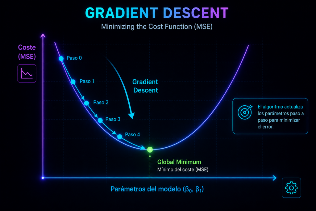
Bring back the image from Part 2: the cost function (the MSE) was a smooth, bowl-shaped landscape.
- The horizontal axes represent the model’s parameters: (the intercept) and (the slope).
- The vertical axis represents the error, the MSE.
- The bottom of the bowl is the global minimum: the combination of parameters that produces the best possible line.
Gradient Descent is nothing more (and nothing less) than the algorithm that walks down that landscape until it reaches the lowest point. Everything that follows is just the details of how it takes each step.
2. The gradient: the compass that points uphill
Before moving, the model needs to answer a very specific question:
If I tweak or a little, does the error go up or down? And by how much?
That information is exactly what the gradient gives you. Mathematically, it’s a vector made up of the partial derivatives of the cost function with respect to each parameter:
But in human terms the idea is very simple:
The gradient tells you the direction in which the error increases the fastest, and how steeply.
Here’s the elegant part: since we want the exact opposite, to decrease the error, all we have to do is move in the opposite direction to the gradient. The gradient points uphill; we walk downhill.
3. The update rule: take a step downhill
Once we know the gradient, the rule for improving is surprisingly short:
Where:
- is the parameter we’re adjusting ( or ),
- is the learning rate (the step size),
- is the slope of the error with respect to that parameter.
In plain English, the formula says this:
New value = current value − (slope of the error) × (step size)
And that’s it. That’s the whole algorithm. All the model does is apply this subtraction over and over, adjusting and at the same time, until the error stops dropping.
One lovely detail about this formula: the slope acts as an automatic brake. When you’re far from the bottom, the slope is steep and the steps are long; as you get closer to the minimum, the slope flattens out, the steps shorten on their own, and the model «lands» gently. Nobody has to tell it when to slow down: the geometry of the landscape does it for you.
4. The learning rate: the most delicate dial
The learning rate controls how far you move with each step, and it’s probably the hyperparameter that causes the most headaches in all of ML. There are three scenarios:
| Learning rate | What happens |
|---|---|
| Too small | The model descends fine, but at a snail’s pace. It can take forever to reach the bottom. |
| Too large | The steps are so long that the model overshoots, bounces from one wall of the bowl to the other, and diverges (the error grows instead of shrinking). |
| Just right | The model descends quickly and smoothly, and settles cleanly into the minimum. |
The mental image is walking down a staircase: with tiny steps it takes you an eternity, but if you try to take three steps at a time you end up flat on the floor. Finding the balance, usually by trying out several values, is one of the most practical skills you’ll pick up in Machine Learning.
5. Visual intuition: walking down a hill in the fog
This is, for me, the best way to picture it. Imagine you’re on a hill at night, in thick fog, with a flashlight that only lights up the ground right in front of your feet.
You can’t see the whole landscape. You don’t know exactly where the bottom is. The only things you can sense are:
- the steepness of the ground where you’re standing,
- which way it slopes downward,
- and what step size you want to take.
With that limited information, your strategy is just common sense:
- you look at the slope under your feet,
- you take a step in the direction that goes down,
- you check the slope again,
- you take another step,
- you repeat.
Step by step, without ever seeing the full map, you end up reaching the bottom of the valley. That’s Gradient Descent: a «blind» algorithm that only needs to know the local slope to find its way. And the best part (thanks to the fact that the linear regression landscape is convex, as we saw in Part 2) is that this bottom is always the same one, the global minimum, no matter where you start your descent.
6. Why this algorithm matters far beyond regression
Here’s an honest question you might be asking yourself: Linear Regression has an exact solution (there’s a closed-form formula that gives you the best and in one shot, no iteration needed). So why bother with Gradient Descent at all?
The answer is that linear regression is the perfect excuse to learn it, because almost no other model gets that luxury. The moment the problem gets more complex, the magic formula disappears and only one option remains: walk down the hill, step by step. Gradient Descent is the engine that trains:
- logistic regression,
- support vector machines (SVMs),
- neural networks,
- deep learning,
- the transformers behind today’s language models,
- and, in general, any model trained with backpropagation.
That’s why it’s no exaggeration to say that Gradient Descent is the engine of modern AI. If you truly understand this algorithm in the simple case of a straight line, you already grasp the essential mechanics by which a model with billions of parameters learns. The scale changes, but the idea is exactly the same.
7. Variants of Gradient Descent (a quick look)
Not every version of the algorithm takes its step the same way. The difference lies in how much data the model looks at before updating the parameters:
| Variant | How much data per step | Character |
|---|---|---|
| Batch Gradient Descent | All the data at once | Very stable, but slow and memory-heavy on large datasets. |
| Stochastic Gradient Descent (SGD) | A single data point per update | Very fast, but «noisy»: the path to the bottom zigzags. |
| Mini-Batch Gradient Descent | Small batches (32, 64, 128…) | The perfect balance between speed and stability. It’s what deep learning uses in practice. |
An intuitive way to see it: batch is like studying the whole map before every step (safe but slow), SGD is like taking a step trusting only a quick glance (fast, but you trip sometimes), and mini-batch is the sensible middle ground that almost everyone ends up using. Later in the series we’ll devote some space to these variants in detail.
In short
- Gradient Descent is the algorithm that reduces a model’s error iteratively.
- The gradient points toward where the error increases; the model moves in the opposite direction.
- The update rule is a simple subtraction: current value − slope × step size.
- The learning rate controls the step size, and tuning it well is key.
- By repeating the process, the model descends to the global minimum (guaranteed, because the landscape is convex).
- This algorithm is the engine that trains almost every modern model, from logistic regression to transformers.