


Logistic Regression (Part 7): Regularization in Classification
When probabilities start to misbehave, regularization becomes essential.
In Parts 1 through 6 we learned how to fit straight lines, how to bend the model when we needed to, and how to tame overfitting by penalizing coefficients with Ridge, Lasso, and Elastic Net. We did all of that on linear regression, where the model predicts continuous numbers.
Today we take the natural next step: carrying those same ideas into classification. And the good news, which we’ll see throughout the article, is that almost everything you already know transfers directly. What we predict changes and the loss we measure changes, but the regularization and training machinery is the same one you already master.
1. Why logistic regression needs regularization even more than linear regression
Logistic regression doesn’t predict just any number: it predicts a probability, a value between 0 and 1. To pull this off, it takes the same old linear combination and squashes it with the sigmoid function:
Thatzis exactly the same line (or hyperplane) as always. The sigmoid only takes care of turning any real number into something interpretable as a probability: it pushes very negativezvalues toward 0 and very positive ones toward 1.
And that’s precisely where the problem lies. The sigmoid saturates at the extremes:
- if
zis very large and positive →ŷ ≈ 1 - if
zis very large and negative →ŷ ≈ 0
In those flat zones the curve barely changes even whenzchanges a lot, so its slope (the gradient) becomes tiny. When that happens, two bad things occur at once: learning slows down because the gradient steps lose their strength, and the model becomes dangerously overconfident, declaring «this is class 1 with 99.9% probability» even when it’s wrong.
And what pushesztoward those enormous values? Enormous coefficients. If the β’s grow unchecked,zblows up, the sigmoid saturates, and the model memorizes the noise in the training set instead of learning the general pattern.
It’s exactly the same overfitting mechanism we saw in Part 6, but here it has an extra nasty side effect: on top of generalizing poorly, it wrecks the quality of the probabilities. That’s why regularization isn’t a luxury in classification but almost a necessity.
2. The loss changes: goodbye MSE, hello Log-Loss
In linear regression we measured error with MSE. In logistic regression we swap it for the log-loss (or binary cross-entropy), which measures how good the predicted probabilities are:
It looks more intimidating than it is. Read it in pieces: for an example whose true class is1(yᵢ = 1), only the first term survives,log(ŷᵢ), which punishes you more the lower the probability you assigned to the correct class. For a class0example, the second term survives. In both cases the idea is the same: it penalizes being wrong, and it penalizes being wrong with high confidence brutally. Predicting 0.99 for something that was class 0 sends the loss shooting toward infinity.
Why not stick with MSE? For several reasons that reinforce each other:
- MSE combined with the sigmoid is not convex, so gradient descent could get stuck in local minima.
- Log-loss is convex, which gives us back the comfortable guarantee from Part 4: a single global minimum.
- Log-loss handles probabilities well and heavily punishes unjustified confidence, exactly what MSE fails to do.
- And it’s not an arbitrary invention: it arises naturally from maximum likelihood (MLE). Maximizing the probability of having observed your data is exactly equivalent to minimizing the log-loss.
The key point for this article: changing the loss doesn’t change how we regularize. The penalty gets added on top just like before.
3. L2, L1, and Elastic Net regularization in logistic regression
The recipe is identical to Part 6: we take the loss and add a term that punishes large coefficients. It’s just that now the base loss is the log-loss.
Ridge (L2)
It penalizes the square of the coefficients, which pushes all of them toward small values without driving them to zero. In classification this has a very concrete benefit: by keeping the β’s contained, it preventszfrom blowing up and therefore prevents the sigmoid from saturating. The result is a smoother, more stable decision boundary, with all variables still present.
Lasso (L1)
It penalizes the absolute value, and that has the characteristic effect of driving some coefficients to exactly zero. In practice, Lasso performs variable selection: it discards the irrelevant ones on its own. The model ends up simpler, with a cleaner decision boundary that’s much easier to interpret (you can say which variables actually matter).
Elastic Net
It combines both penalties. It’s the option to reach for when you have many variables correlated with each other: Lasso on its own tends to pick one from the group almost at random and discard the rest, while the L2 part of Elastic Net spreads the weight more stably. You get Lasso’s variable selection and Ridge’s smoothness.
| Method | What it does to coefficients | When it shines |
|---|---|---|
| Ridge (L2) | Shrinks them, none go to zero | Many useful variables; you want stability |
| Lasso (L1) | Zeroes out the irrelevant ones | You want a simple, interpretable model |
| Elastic Net | A blend of both | Many correlated variables |
4. How it trains: same engine, new loss
Here comes the most satisfying part, and it’s worth pausing on. The update rule is the same as always:
And the beautiful thing is what pops out when you compute the derivative of the log-loss with the sigmoid. After simplifying (the ugly terms cancel out in an almost magical way), the derivative comes out like this:
Look closely: it’s exactly the same form as the linear regression in Part 4. «Error times the variable, averaged.» The only difference is that nowŷᵢcomes from the sigmoid instead of a direct line. That’s the real reason we say the mechanism is identical: it’s not just that it «resembles» it, it’s that the gradient formula matches literally.
So the full update, with L2 regularization for example, comes out as:
The only genuinely new thing compared to Part 6 is thatŷpasses through the sigmoid and that this sigmoid can saturate. The L1/L2 penalty behaves just as you already know.
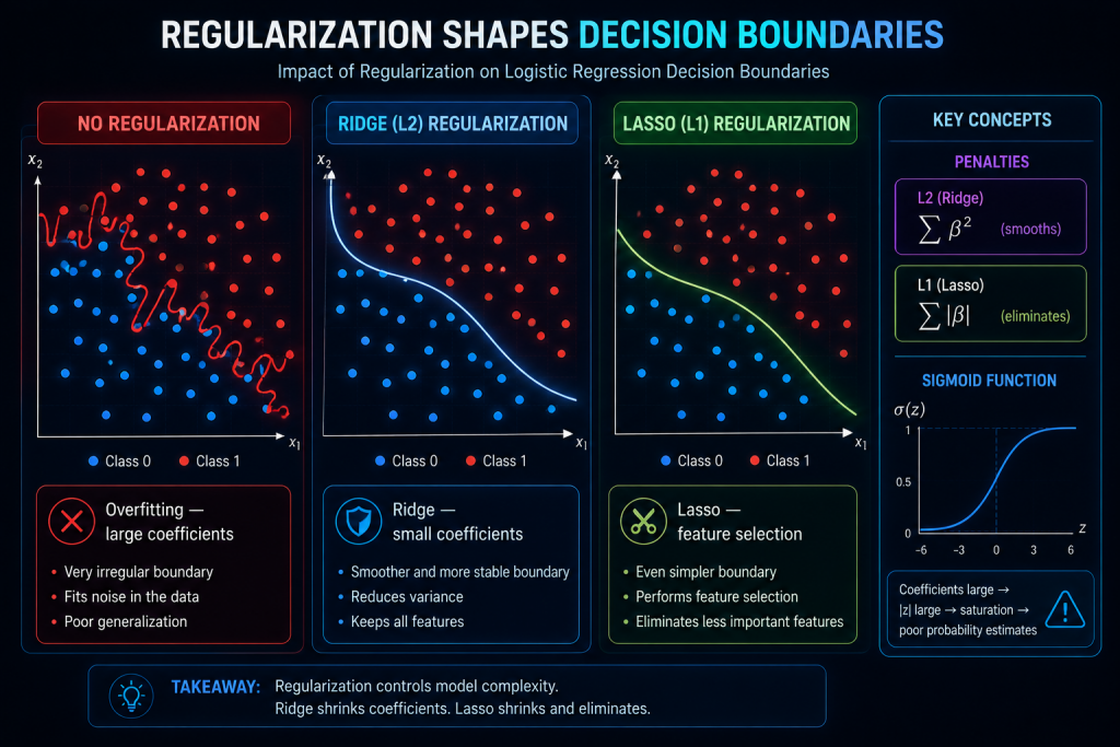
5. What happens geometrically: three boundaries, three behaviors
In classification, the model doesn’t draw a line running through the points but a decision boundary: the line (or curve) that separates one class from another. Regularization acts directly on the shape of that boundary.
Picture a problem with two intermingled classes:
- Without regularization: with the freedom to let coefficients grow, the boundary twists and zigzags trying to capture every individual point, noise included. It fits perfectly on training data and fails on new data. Textbook overfitting.
- With Ridge: by containing the coefficients, the boundary smooths out. It stops chasing isolated points and captures the general trend. More stable, generalizes better.
- With Lasso: on top of smoothing, it eliminates the variables that don’t contribute, which simplifies the boundary even further by reducing the dimensions that actually take part.
The underlying intuition is that large coefficients = twisted boundaries = saturated sigmoid, and all three forms of regularization (Ridge, Lasso, and Elastic Net) attack exactly that root by keeping the coefficients in check.
6. When to use regularization in classification (and when not to)
It’s not a tool you should turn on by default every time. The point is to recognize the signals.
Turn it on when:
- You have many features, especially if there are more of them than training examples.
- There’s multicollinearity (variables highly correlated with each other).
- The decision boundary looks too complex or unstable.
- You observe enormous coefficients or suspiciously extreme probabilities (0.999, 0.001).
- The validation error is much larger than the training error: the classic signature of overfitting.
Think twice when:
- You have lots of data and few variables: the model has little room to overfit already.
- The model already generalizes well: don’t fix what isn’t broken.
- The problem is lack of expressiveness, not excess: if the model falls short (underfitting), regularizing only makes things worse, because it ties its hands even more.
In practice, the knob you tune isλ(or its inverse,C, in tools like scikit-learn, where a largeCmeans little regularization). You choose it with cross-validation, trying several values and keeping the one that generalizes best.
7. In summary
- Logistic regression predicts probabilities via the sigmoid, not continuous numbers.
- The sigmoid saturates when coefficients grow: tiny gradients, overconfidence, and worse generalization.
- We swap MSE for the log-loss, which is convex, punishes unjustified confidence, and is born from maximum likelihood.
- Ridge smooths the coefficients, Lasso zeroes them out and does variable selection, and Elastic Net combines both for correlated variables.
- Training is still gradient descent, and its formula matches literally the one from Part 4: «error times variable, averaged.»
- Regularization is the key to achieving stable decision boundaries and reliable probabilities.
With this we close the loop on the whole series: the same three ideas (a loss, a gradient, and a penalty) work both for predicting numbers and for classifying. The only thing that changes between one problem and the other is the function wrapping the output and the loss you measure. The engine, always the same.