





K‑NN and Naive Bayes
Two classic classifiers, simple and effective, that work for completely different reasons
In classification there are models that learn complex boundaries, like SVMs or trees. They learn, they fit, they optimize. And then there are K‑NN and Naive Bayes, two radically different approaches from each other, yet equally useful when you want something quick to understand, easy to implement, and surprisingly competitive on many real-world problems.
What’s interesting is why they work, because they do it from opposite philosophies. One reasons with geometry (who do you resemble?) and the other with probability (what is most likely?). Understanding that difference is understanding half of a classification course. Let’s get straight to the point.
K‑NN: classifying by neighborhood
Let’s start with an image. Imagine you just moved to a new city and you want to know whether a neighborhood is quiet or noisy. What do you do? You look at your nearest neighbors. If the five people next door say it’s quiet, you bet on quiet. You don’t need an urban planning study or a statistical model: you trust who’s close to you.
That’s exactly K‑NN, and that’s why it’s so intuitive.
The first thing that surprises people about K‑NN (K‑Nearest Neighbors) is that it doesn’t train anything. It doesn’t learn weights, it doesn’t fit coefficients, it doesn’t optimize a loss function. That’s why it’s called a lazy learner: it does no work in advance, it simply stores all the data and waits. All the effort happens at prediction time.
When a new point arrives, it does just one thing:
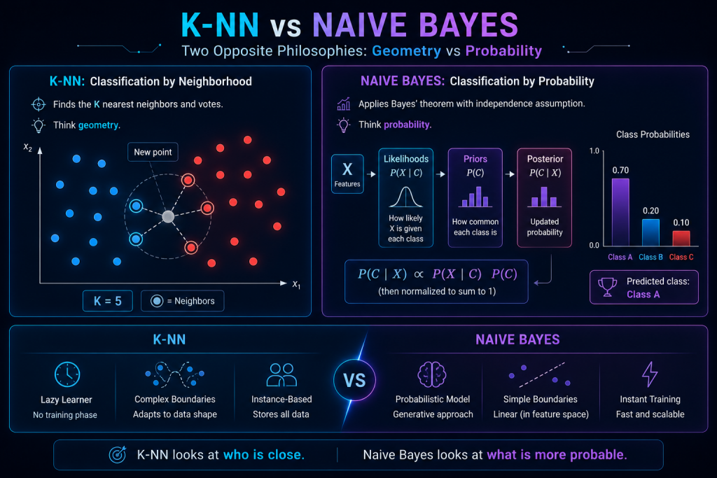
It finds the K nearest points in the dataset and votes for the majority class.
That simple.
A numerical example
Imagine you classify fruit as apple or orange based on two features: weight and skin roughness. A new fruit arrives and you compute its 5 nearest neighbors:
| Neighbor | Distance | Class |
|---|---|---|
| 1 | 0.8 | Apple |
| 2 | 1.1 | Orange |
| 3 | 1.3 | Apple |
| 4 | 1.6 | Apple |
| 5 | 1.9 | Orange |
With K = 5, we count: 3 apples versus 2 oranges. Apple wins. Done. There’s no more magic than counting votes among the neighbors.
How does it decide who is «close»?
It uses a distance metric. The most common ones:
- Euclidean: the good old «straight-line» distance. The default option.
- Manhattan: sums the differences axis by axis, like moving through the streets of a grid-based city.
- Cosine: measures the angle between two vectors, not their length. It’s the queen when you work with text or embeddings.
The K parameter: the overfitting dial
The value of K controls how much «detail» the model looks at, and choosing it well is almost the whole game:
- K = 1: the model copies the class of the nearest neighbor. Fast, but very sensitive to noise: a single mislabeled data point can ruin your prediction.
- Large K: the boundary smooths out. Less overfitting, but a greater risk of ignoring fine details and blurring small classes.
A practical tip: always use an odd K in two-class problems, to avoid ties in the vote.
Advantages
- Requires no training.
- Works well with complex, non-linear boundaries.
- Very intuitive and easy to explain.
- Excellent as a baseline: if your fancy model can’t beat K‑NN, something is off.
Disadvantages
- Slow with lots of data: each prediction forces you to scan the whole dataset looking for neighbors.
- Sensitive to the scale of the variables: if one variable ranges from 0 to 1 and another from 0 to 10,000, the second dominates the distance. That’s why normalizing is mandatory.
- Suffers from the curse of dimensionality: in many dimensions, all points end up looking equally far apart and the concept of a «close neighbor» loses meaning.
Naive Bayes: classifying by probability
Naive Bayes is the opposite of K‑NN. It doesn’t look at neighbors, it doesn’t compute distances, it doesn’t search for geometric patterns. Instead, it reasons like a detective: it gathers clues and calculates which explanation is most likely.
Think of a doctor facing a patient with fever, cough, and a sore throat. They don’t measure «distances»: they think «given these symptoms, which illness is most likely?». They combine the general frequency of each illness with the probability that each one produces those symptoms. That’s Naive Bayes.
Formally, the model estimates the probability of each class given the features:
And it does so with Bayes’ theorem:
In plain English, each piece has a name and a very concrete meaning:
- $P(C)$ is the prior: how common the class is to begin with (how many emails are spam in general?).
- $P(X \mid C)$ is the likelihood: how probable it is to see these features if it were that class (does the word «free» show up in spam?).
- $P(C \mid X)$ is the posterior: what we want, the probability of the class once we’ve seen the clues.
Why is it called «naive»?
Because it makes a very strong, almost shameless assumption:
All features are independent of each other.
That is, it assumes the word «free» and the word «offer» appear in an email with no relation whatsoever, when in reality they tend to go hand in hand. That assumption is almost never true in the real world. Hence naive.
And why does it work so well if the assumption is false?
This is the fascinating part. Even though the individual probabilities are miscalculated by ignoring correlations, to classify we don’t need the exact probability: we only need the correct class to come out with the highest probability. And for that, approximate independence is usually enough. The result is a model that is:
- blazing fast,
- stable even with little data,
- and surprisingly accurate, especially with text.
A numerical example (spam detection)
Suppose you want to classify an email that contains the word «free». You know that:
- 40% of emails are spam → $P(\text{spam}) = 0.4$
- 80% of spam emails contain «free» → $P(\text{free} \mid \text{spam}) = 0.8$
- Only 10% of normal emails contain «free» → $P(\text{free} \mid \text{not spam}) = 0.1$
We compare the two paths (the numerators of Bayes’ formula):
- Spam: $0.4 \times 0.8 = 0.32$
- Not spam: $0.6 \times 0.1 = 0.06$
Since 0.32 is much larger than 0.06, the model classifies the email as spam. And notice: we didn’t even need to compute the denominator, because all we care about is which one wins.
Common variants
Naive Bayes comes in several flavors depending on the type of data:
- Gaussian NB → for continuous data (assumes it follows a bell curve).
- Multinomial NB → for text with word counts (bag of words). It’s the classic for spam filtering.
- Bernoulli NB → for binary variables (the word appears or it doesn’t).
Advantages
- Extremely fast to train and to predict.
- Works very well with text: email classification, sentiment, topics.
- Requires very little data to give decent results.
- Outputs probabilities directly, not just a label.
Disadvantages
- The independence assumption rarely holds completely.
- It doesn’t capture interactions between variables.
- It produces relatively simple boundaries.
- It struggles with never-before-seen words/categories (fixed with Laplace smoothing, a small adjustment that avoids multiplying by zero).
Two opposite philosophies, at a glance
Before comparing when to use each one, it’s worth seeing at once just how different they are under the hood:


One asks «who do I resemble?». The other, «what am I most likely to be?». Same goal, opposite paths.
K‑NN vs Naive Bayes: when to use each
| Situation | Better choice |
|---|---|
| Data with geometric structure | K‑NN |
| Text, emails, documents | Naive Bayes |
| Small dataset | Both |
| Large dataset | Naive Bayes |
| Complex, non-linear boundaries | K‑NN |
| You need extreme prediction speed | Naive Bayes |
| Highly correlated variables | K‑NN |
| Very high dimensionality (e.g. thousands of words) | Naive Bayes |
The quick mental rule: if your data «lives in a space» where closeness makes sense, go with K‑NN. If you have many count-type features (especially text) and you want something instant, go with Naive Bayes.
In summary
- K‑NN classifies by neighborhood: it stores the data, finds the K nearest points, and votes. It doesn’t train; all the work happens at prediction time.
- Naive Bayes classifies by probability: it applies Bayes’ theorem assuming (naively) that the variables are independent.
- Both are simple, fast, and excellent as a baseline before moving on to heavier models.
- They shine in different contexts: K‑NN for geometry, Naive Bayes for text.
- And the best part: understanding these two gives you the intuition for the two great families of classification (distance-based and probability-based) before you jump into more complex models.