





SVM: Hyperplane, Margin, and Kernel
The model obsessed with finding the perfect boundary
We’ve already seen models that classify by proximity, like K‑NN, asking «who do I look like?». Others do it by probability, like Naive Bayes, asking «what’s most likely?». And others do it through chained questions, like decision trees.
SVMs do something different: they draw boundaries.
But careful, not just any boundary. Imagine you have to paint a line on the ground to separate two groups of kids in a playground. You could paint it hugging one group, or crooked, or by eye. An SVM wouldn’t: an SVM would look for the line that leaves the most free space possible on both sides, so nobody steps on it by accident. It is, in essence, an architect obsessed with geometry, incapable of settling for a boundary that’s «good enough.»
Let’s get to the point.
What is an SVM?
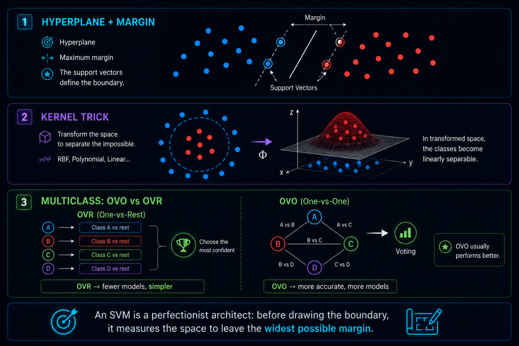
An SVM (Support Vector Machine) tries to find a hyperplane that separates two classes.
The word «hyperplane» sounds scarier than it should. It’s really just the fancy name for «the boundary,» and it changes shape depending on how many dimensions you have:
- In 2D it’s a simple line.
- In 3D it’s a plane (like a sheet of paper floating in the air).
- In higher dimensions it’s a surface we can no longer draw, but that works just the same.
Now, the point isn’t just to separate. Anyone can split two groups with a line. What makes the SVM special is this:
The SVM looks for the hyperplane that leaves the largest possible margin between the classes.
That margin is the distance between the boundary and the closest points of each side. And here’s the golden rule: the bigger the margin, the more robust the boundary.
The intuition: separating with the maximum margin
Picture two groups of points on a plane, some blue and some red, clearly apart. There are infinitely many lines that could separate them: a slanted one, one almost touching the reds, one almost touching the blues… they all «work» on paper.
But only one leaves the largest possible gap between both groups, like a hallway wide enough for a car to drive through. That’s the line the SVM wants.
Why is it so obsessed with the wide hallway? Think of it this way: if a new point shows up tomorrow, slightly shifted by noise or chance, a boundary with a wide margin absorbs the bump without making a mistake. A boundary glued to one group, on the other hand, gets crossed at the slightest push. That’s why a large margin generalizes better and is less sensitive to noise: it leaves a safety cushion.
The «support vectors»: the points that call the shots
Here comes a lovely and very counterintuitive detail.
Of all your data, do you know which points the SVM actually uses to decide where the boundary goes? Only a handful. The points sitting right at the edge of the hallway, the ones that «touch» the margin, are the so‑called support vectors.
And they’re the only ones that truly matter:
- If you remove a support vector, the boundary shifts.
- If you remove any other point (one of the crowd, far from the boundary), absolutely nothing happens.
It’s like pitching a tent: the shape is held up by the stakes at the edges, not by the fabric in the middle. Pull out a stake and the whole tent sags; crumple the fabric in the center and nothing changes. The SVM is a model that only learns from the critical points, and ignores the rest. That’s what makes it so efficient.
What if the data can’t be separated with a line?
So far so nice… but the real world almost never lets itself be split with a straight line. This is where the cleverest part of SVMs comes in: the kernel.
The kernel is a function that lets the SVM work in a higher‑dimensional space without having to compute it explicitly (this last part is known as the kernel trick, and it’s what makes it feasible). In plain terms, it’s as if the SVM said:
«In this plane, the way things are, I can’t separate the classes. But if I lift the data into a higher dimension, suddenly I can.»
The most common kernels are:
- Linear → when the classes are already almost separated on their own. The simplest and fastest.
- Polynomial → adds curves to the boundary.
- RBF (Gaussian) → creates smooth, very flexible boundaries.
- Sigmoid → behaves somewhat like a neural network.
Of all of them, RBF is the most used, because it works surprisingly well on tons of real problems without much fuss. If you’re unsure where to start, start there.
The intuition behind the kernel (without a single formula)
This is the example that makes everything click, so read it slowly.
Picture two concentric circles, like a dartboard: the red points inside, forming the small circle, and the blue points outside, surrounding them. In 2D, on the table, there is no straight line that separates red from blue. Try it in your head: any line you draw leaves reds and blues mixed on both sides.
Now do this trick: grab the red circle in the center and lift it upward, as if you were pulling the middle of a tablecloth and forming a mountain. The reds rise, the blues stay down. And all at once, in that 3D space, you can separate them with a simple horizontal sheet of paper slid between the mountain and the base.
That’s exactly what a kernel does: it transforms the space so an impossible separation becomes trivial. It doesn’t change the data; it changes the point of view.
SVM with more than two classes: OVO vs OVR
There’s a small catch: SVMs were born to separate only two classes (red or blue, yes or no). So how do they cope when you have 4, 10, or 20 classes?
The answer is clever: they break the big problem into lots of small two‑way duels. There are two ways to organize those duels.
1. One‑vs‑Rest (OVR): «me against the world»
For each class, you train an SVM that separates it from all the others combined. With 4 classes (A, B, C, D) you’d have:
- SVM A vs (B, C, D)
- SVM B vs (A, C, D)
- SVM C vs (A, B, D)
- SVM D vs (A, B, C)
At prediction time, each SVM says how confident it is, and the most confident one wins.
It’s like asking four specialists, each of whom only knows how to recognize their class: «is this an A or not?», «is this a B or not?»… You go with whoever answers most emphatically.
2. One‑vs‑One (OVO): «everyone against everyone»
Here you train an SVM for each pair of classes. With 4 classes you get 6 duels:
- A vs B, A vs C, A vs D
- B vs C, B vs D
- C vs D
At prediction time, each model votes for one of its two assigned classes, and the class with the most votes wins. It’s an everyone‑against‑everyone tournament, like a round‑robin league where the team with the most wins takes the trophy.
Which one to choose?
| One‑vs‑Rest (OVR) | One‑vs‑One (OVO) | |
|---|---|---|
| Number of models | K (one per class) | K(K‑1)/2 (one per pair) |
| How it decides | The most confident SVM | The most voted class |
| Data per model | Imbalanced (1 class vs many) | More balanced (1 vs 1) |
| Advantage | Fewer models, simple | More precise boundaries |
| Drawback | Gets imbalanced if a class is small | Many models if there are many classes |
To see the jump at a glance: with 10 classes, OVR trains 10 models, while OVO trains 45. It looks like OVR wins by a landslide… but each OVO model is smaller, faster to train, and sees more balanced data, so in practice OVO tends to work better. In fact, it’s the default approach in many libraries, like scikit‑learn.
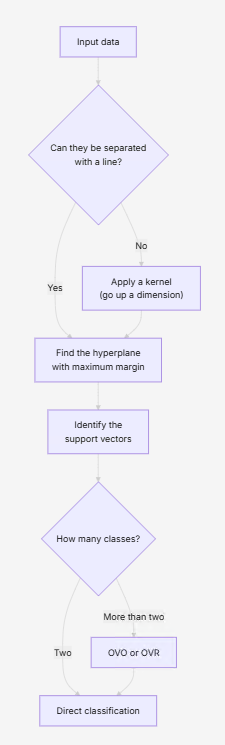
The full SVM flow, at a glance
Advantages of SVMs
- They handle complex boundaries without breaking a sweat, thanks to kernels.
- They’re very robust to noise, because the wide margin acts as a cushion.
- They focus on what matters: only the support vectors.
- They work well in high‑dimensional spaces, where other models get lost.
- They’re excellent with small or medium, well‑defined datasets.
Disadvantages
- They don’t scale well to huge datasets: with millions of examples, training gets heavy.
- Choosing the kernel and its parameters can be tricky and takes experimentation.
- They’re less interpretable than a tree or a regression: it’s harder to explain why they decided something.
- Training can be slow.
It’s precisely because of these limitations (especially scale) that today, for massive problems, people usually turn to other approaches. But on their home turf (few data, well defined, tough boundaries) they’re still unbeatable.
When to use an SVM?
- When the classes can’t be separated with a straight line.
- When you have few data points, but well defined ones.
- When you need a robust boundary that won’t break under noise.
- When you want a powerful model without getting into neural networks.
In short
- An SVM looks for the hyperplane with the maximum margin, the widest possible hallway between the classes.
- The support vectors are the handful of edge points that define the boundary; the rest don’t count.
- The kernel lets you separate impossible classes by changing the space, not the data (remember the dartboard and the mountain).
- For multiple classes: OVR is simple and uses few models; OVO is more precise and usually wins in practice.
- SVMs are powerful, robust, and brilliant on small or medium datasets.
And if you take away just one image: an SVM is that perfectionist architect who, before drawing a single line, measures the space on both sides to leave the widest possible hallway. That obsession with the margin is exactly what makes it so good.