





Unsupervised Learning — Clustering
DBSCAN: the algorithm that finds groups without asking for permission
The model that doesn’t need you to tell it how many groups there are… and that spots the noise all on its own.
In the previous chapter we met K‑means, a tidy, almost polite algorithm: you tell it how many groups you want, it looks for centers, shuffles points around, and hands you nice, round, well‑defined clusters. All very clean, all very predictable.
DBSCAN is the exact opposite.
DBSCAN is a rebel. It doesn’t want you to tell it how many groups there are. It doesn’t want perfect shapes. It doesn’t want you to mark out the path.
The only thing it cares about is density. It hunts for zones where points sit close together, packed tight, forming «neighborhoods.» And if it finds a lone point, stranded in the middle of nowhere… it flags it as noise without blinking.
Today you’re going to meet the algorithm that discovers groups exactly where K‑means throws up its hands and gives up.
The example that follows us around
Let’s stick with our online store, the same one from the previous chapter. You have thousands of customers, and for each one you know just two things: how much they spend per month and how many times they buy.
But this time there’s an awkward detail: some customers don’t look like anyone else. Alongside the compact group of loyal buyers and the group of occasional shoppers, a handful of truly odd cases sneak in:
- one who buys 40 times a month but spends peanuts (a reseller? a bot?),
- another who buys just once a year but drops a fortune,
- and another who, quite simply, follows no recognizable pattern at all.
K‑means would try to cram all three into some group even though they don’t fit, dragging its centers around and wrecking the segmentation in the process. DBSCAN won’t. DBSCAN looks at them, decides they don’t belong to any neighborhood, and sets them aside as noise. And that ability to say «this doesn’t belong» is exactly its superpower.
The intuition: DBSCAN looks for «neighborhoods»
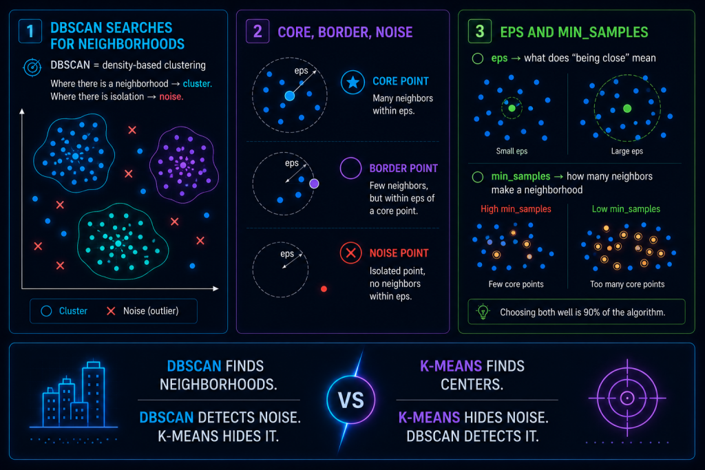
K‑means looked for centers. DBSCAN looks for dense zones.
Picture a city map seen from a plane. There are neighborhoods where the houses are packed against one another, streets bursting with life, squares full of people. And then there are empty lots, vacant plots, isolated houses out in the middle of the fields.
DBSCAN does exactly that:
- where it sees lots of people together → it says «this is a cluster,»
- where it sees a single, lonely house → it says «this is noise.»
It’s an algorithm that thinks like a city planner: it walks the map and marks where there’s neighborhood life and where there’s only silence.
The three types of points
To do that job, DBSCAN sorts every point into one of three categories. It’s easier than it sounds if you keep picturing the city map:
- Core point. A point with lots of neighbors nearby. It’s the heart of the neighborhood, the central square where everyone gathers.
- Border point. A point that sits right next to a core but has few neighbors of its own. It’s the house on the edge of the neighborhood: still part of it, but already almost touching the countryside.
- Noise point. An isolated point with too few neighbors. It’s the house lost in the middle of nowhere, with no neighborhood to belong to.
This classification is what makes DBSCAN so powerful: it detects outliers naturally, as a side effect of how it works, without you ever having to go looking for them.
The two key parameters: eps and min_samples
The neat part is that, to do all of this, DBSCAN only needs two numbers:
eps→ the neighborhood radius. It answers the question «what does it mean to be close?». It’s how far you look around each point to count its neighbors.min_samples→ how many neighbors it takes to be a core. It answers «how many houses make a neighborhood?».
The magic happens when you combine the two. For example, withmin_samples = 4: a point becomes a core if it finds at least 4 neighbors within itsepsradius. If it has fewer neighbors but sits within the radius of a core, it’s a border point. And if it meets neither condition, it’s noise.
The balance between the two changes everything:
- if
epsis too small → it only detects ultra‑compact neighborhoods and marks almost everything else as noise, - if
epsis too large → it merges zones that shouldn’t go together and ends up with one mega‑cluster that swallows everything, - if
min_samplesis high → it demands a lot of density, so it forms few, very strict clusters, - if
min_samplesis low → it forms clusters far too easily, and even the noise starts to look like a group.
Choosing these two numbers well is 90% of the work with DBSCAN. A common trick for nailingepsis to sort every point by the distance to its nearest neighbor and look for the «elbow» in that curve, just like we did with the elbow method in K‑means.
Why is DBSCAN so different from K‑means?
DBSCAN breaks, one by one, almost every rule of K‑means:
- It doesn’t need you to tell it K. You don’t have to guess how many groups there are; it discovers them by itself from the density.
- It detects weird shapes. K‑means only gets along with round little groups. DBSCAN finds curved, elongated clusters, ones with holes… shapes that look like snakes, moons, or coffee stains.
- It detects noise. K‑means forces everyone into some group no matter what. DBSCAN leaves out whoever doesn’t fit.
- It doesn’t rely on centroids. There are no centers to reposition over and over. There’s only density, neighbors, and radii.
To see it at a glance:
| K‑means | DBSCAN | |
|---|---|---|
| Do you have to pick the number of groups? | Yes (you choose K by hand) | No (it discovers them itself) |
| Shapes it detects | Only round and compact | Any shape: curved, elongated, with holes |
| What it does with outliers | Forces them into a group | Sets them aside as noise |
| Parameters to tune | K | epsandmin_samples |
| Speed on huge datasets | Very fast | Slower |
| Sensitive to uneven densities | Less so | Yes, very (its Achilles’ heel) |
Pros and cons of DBSCAN
Like everything in machine learning, DBSCAN isn’t magic: it shines in some scenarios and sinks in others. It’s worth being clear on that before you unleash it on your data.
| ✅ Pros | ❌ Cons |
|---|---|
| You don’t have to choose K upfront | Choosingepscan be tricky and takes trial and error |
| Detects outliers automatically | Fails when groups have very different densities |
| Works with arbitrarily shaped clusters | Scales worse than K‑means on huge datasets |
| Very intuitive if you think in terms of density | Sensitive to scale: you absolutely must normalize |
| Ideal for data with natural «neighborhoods» | A singleepswon’t do if some neighborhoods are dense and others sparse |
About that last drawback: if your data has some very tight zones and others very loose, a singleepscan’t please both, and that’s where DBSCAN starts to stumble. For those cases there are variants like HDBSCAN, but that’s another story.
When to use DBSCAN and when not to
So you don’t get it wrong, here’s a visual summary of when DBSCAN is your ally and when you’re better off looking at another algorithm:
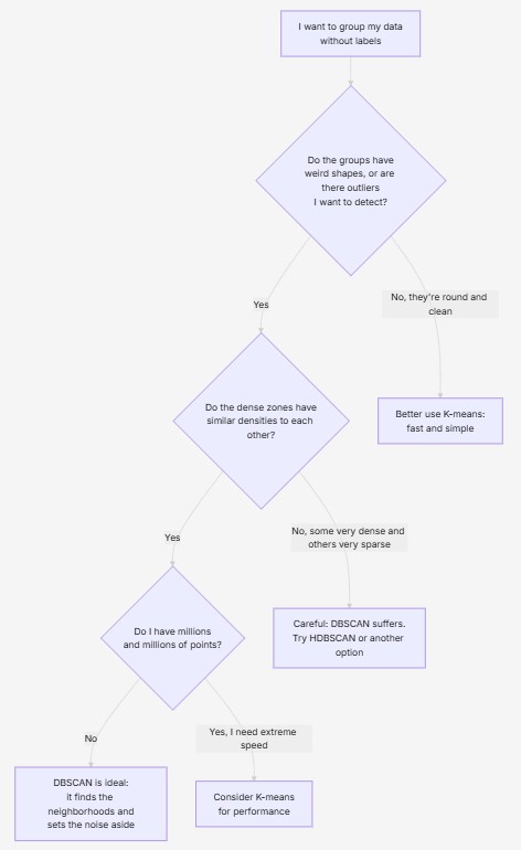
In short, DBSCAN is your friend when clusters have weird shapes, when there are outliers you want to catch, when you don’t know how many groups there are, or when K‑means hands you absurd results. And it’s not your friend when densities are wildly uneven, when you need extreme speed over millions of points, or when the data simply has no density structure.
In summary
- DBSCAN groups unlabeled data by hunting for dense zones rather than centers.
- You don’t need to tell it how many groups there are: it discovers them from the density.
- It classifies each point as core, border, or noise, and so it detects outliers naturally.
- It depends on only two parameters,
eps(what counts as close) andmin_samples(how many neighbors make a neighborhood), and choosing them well is nearly the whole job. - It finds shapes K‑means could never detect, but it struggles when densities are very uneven.