




The lifecycle of a Machine Learning model: from experiment to production
How a model goes from a test in a notebook to generating value in the real world
The complete journey from raw data to production monitoring.
For much of this series we’ve dissected models: decision trees, neural networks, Transformers, LLMs, and multimodal systems. We’ve opened up their guts to understand how they think.
But there’s an uncomfortable truth that every professional discovers, almost always the hard way:
A model that works beautifully in a notebook is worth absolutely nothing.
It can reach 99% accuracy. It can generate brilliant text. It can recognize tumors better than a veteran radiologist. And yet, it can fail spectacularly the moment it touches the real world.
The reason is simple and counterintuitive:
Machine Learning doesn’t end when training finishes. That is precisely where the hard part begins.
Because a useful model isn’t a frozen algorithm in a file. It’s a living system. And like everything that’s alive, it needs to feed, adapt, and evolve… or it dies.
1. The great misunderstanding: believing training is the finish line
When we take our first steps in Machine Learning, we imagine a clean, linear, romantic process:

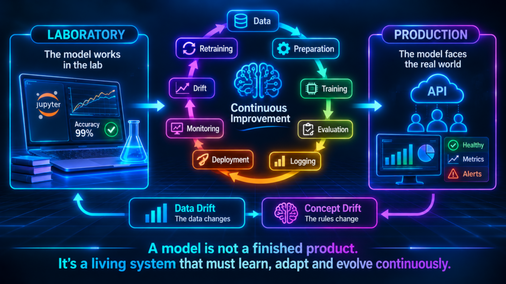
The reality of a production project is far less glamorous and quite a bit more circular. It looks more like this:

The restaurant analogy. Training a model is like cooking one spectacular dish a single time at a cooking contest. But running a restaurant (production) is another story: you have to buy fresh ingredients every day, keep the quality constant across hundreds of diners, adapt the menu when tastes change, and make sure dish number 5,000 tastes just as good as the first. Training is only one stage within a much longer cycle.
2. Phase 1 — Data: the fuel that determines everything
It all starts here. Not with the algorithms, not with PyTorch or TensorFlow. With the data.
The golden rule is relentless and has no exceptions:
A model’s quality can never exceed the quality of the data it receives.
It’s the famous Garbage In, Garbage Out principle. You can have the most sophisticated architecture on the planet, but if you feed it dirty, biased, or incomplete data, you’ll get garbage predictions delivered with alarming confidence.
This phase is home to the least glamorous and, at the same time, most decisive work:
- gathering sources
- cleaning and handling null values
- removing duplicates
- feature engineering
- labeling
The stat that surprises everyone: various industry surveys (such as those by Anaconda or Forbes) estimate that data scientists spend around 80% of their time preparing and cleaning data, and only 20% on what people imagine as «doing AI.» The sexy part is the tip of the iceberg.
3. Phase 2 — Training: learning from the past
This is the phase everyone knows and the one that grabs the headlines. Here the model examines historical data and extracts patterns from it.
Depending on the problem (regression, classification, clustering, deep learning, or fine-tuning an LLM), it can take anywhere from a few seconds on your laptop to weeks on hundreds of GPUs, costing millions.
But beneath all that variety, the same principle always beats:
The model learns from the past to try to predict the future.
And here lies the seed of almost every problem that will come later: the model implicitly assumes that the future will resemble the past. Spoiler: that’s not always the case.
4. Phase 3 — Evaluation: did it learn, or just memorize?
Before trusting a model, you have to answer the most important question of all:
Did it really understand the problem, or did it simply memorize the exam answers?
That «cramming without understanding» phenomenon is called overfitting: the model nails the examples it already saw, but collapses in front of any new data. It’s like the student who memorizes the textbook’s solutions but fails the moment the wording is slightly changed.
To unmask it, we evaluate it with data it never saw during training, using tools like:
| Technique / Metric | What it tells us in plain language |
|---|---|
| Hold-Out / Cross Validation | Setting aside a «surprise test» the model couldn’t study. |
| Confusion matrix | Where it gets things right and, above all, what kind of errors it makes. |
| Precision | Of everything it flagged as positive, how much really was? |
| Recall | Of all the real positives, how many did it manage to catch? |
| F1-Score | The right balance between Precision and Recall. |
| ROC-AUC | Its overall ability to distinguish between classes. |
Here is where we decide whether the model has permission to leave the lab.
5. Phase 4 — Registry and versioning: the end of chaos
And now a problem appears that doesn’t show up in the tutorials. After dozens of experiments, your folder ends up looking like this:
final_model.pkl
final_model_v2.pkl
final_model_v3_definitive.pkl
final_model_v3_definitive_NOW_FOR_REAL.pkl
final_model_v3_definitive_the_actual_good_one.pkl
Which one was trained on which data? Which gave the best F1? Which is actually in production? Nobody knows. Absolute chaos.
That’s why modern MLOps systems introduce industrial discipline:
- Versioning: each model has a unique, traceable identity.
- Traceability: we know exactly what data and what parameters generated it.
- Metric and artifact logging: everything is stored and comparable.
Tools like MLflow, DVC, or Weights & Biases were born precisely to turn that chaos of loose files into an orderly history, just as Git did with code.
6. Phase 5 — Deployment: the real leap into the void
Here the model leaves the comfortable lab and faces the wild world: real data, real customers, unexpected requests, and real errors that cost money.
Not all models are served the same way. There are three main strategies depending on urgency:
| Deployment mode | How it works | Typical example |
|---|---|---|
| Batch | Processes thousands of records at once, on fixed schedules (e.g. every night). | Product recommendations you see the next day. |
| Real-time (API) | Request → immediate prediction → response in milliseconds. | Approving or denying a card purchase instantly. |
| Streaming | A continuous flow of data generating predictions non-stop. | Anomaly detection in factory sensors 24/7. |
It’s the magic moment: at last, the model starts to generate real value.
7. Phase 6 — Monitoring: all models degrade
And here comes the hardest and most humbling lesson of production:
All models degrade over time. It’s not a possibility: it’s a mathematical certainty.
The world changes. Customers change their habits, new competitors arrive, a pandemic erupts, a law changes. And your model, which learned a faithful portrait of yesterday’s world, becomes a little more obsolete each day.
That’s why you can’t just deploy and forget: you have to constantly watch two types of signals.
- Technical signals: latency (is it responding fast?), error rate, resource consumption.
- Business and quality signals: real accuracy, and above all, whether the distribution of the input data still resembles that of the training set.
8. Drift: when the world leaves your model behind
That degradation has its own name and is the great ghost of MLOps: drift. It comes in two flavors that are worth not confusing.
Data Drift: the input data changes
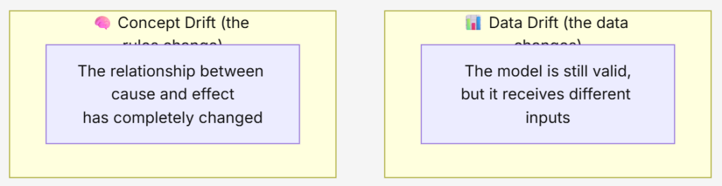
The characteristics of what comes in drift away from what the model knew.
Example: a fraud detector trained on 2023 transactions starts receiving, in 2026, a flood of mobile payments and crypto that barely existed before. The pattern of «normality» has changed beneath its feet.
Concept Drift: the rules of the game change
The most treacherous one: the very relationship between the variables and the outcome breaks.
Classic example: supermarket demand models in early 2020. Overnight, «toilet paper» and «flour» went from predictable products to panic items. The learned rules stopped being true, even though the data «looked» normal.
In both cases, the model keeps working and returning answers with total composure… but it gets things wrong more and more often. It’s a silent and dangerous deterioration.
9. Retraining: teaching it again
When monitoring detects drift, there are only two paths:
- Accept the deterioration (and absorb the losses).
- Retrain the model with fresh information.
The right answer is almost always obvious. Retraining injects the current reality into the system:

And so the cycle starts over. The big strategic question isn’t whether to retrain, but when: every night? every week? only when a drift alarm goes off? That balance between cost and freshness is one of the great challenges of MLOps.
10. The cycle that never ends
Here lies the abysmal difference between an academic exercise and a real production system.
| Academic project | Production system | |
|---|---|---|
| Goal | Publish a good result | Generate sustained value |
| Ending | Ends upon delivery/publication | It never ends |
| Data | Fixed, clean, static | Alive, dirty, changing |
| Success | A good metric in the paper | Reliability over years |
An academic project ends when the result is published. A real Machine Learning system, on the other hand, enters a perpetual loop: train → deploy → monitor → detect drift → retrain → deploy again. And repeat, over and over, for years.
In summary
The complete lifecycle of a modern model covers far more than training:
- gathering and preparing data (the silent 80% of the work),
- training from the past,
- honest evaluation against never-before-seen data,
- registry and versioning to end the chaos of loose files,
- deployment in batch, real-time, or streaming,
- continuous monitoring of the system’s health,
- drift detection before it causes damage,
- and retraining to keep it alive.
The most important lesson of all fits in a single sentence:
A model isn’t a finished product; it’s a living system.
The moment it goes into production isn’t the end of the project… it’s the beginning of its real life.