22 junio 2026

Linear Regression (Part 4)

Coefficient updates: how β₀ and β₁ adjust at every step

In Part 3 we looked at the heart of learning: Gradient Descent. We got the idea of walking down into the valley, the gradient as a compass, and why the learning rate matters. But we left one question hanging in the air, and it’s exactly the one that turns all that theory into something that actually works:

How do the model’s coefficients update exactly?

Because up to now we’ve been speaking in general terms. We know the gradient tells us which direction to move and the learning rate tells us how big each step is. But we still haven’t seen the concrete formulas, the ones the computer runs over and over, thousands of times, so that the line stops being nonsense and starts fitting the data.

Today we close that loop. And you’ll see that, once we take it apart piece by piece, there’s nothing magical going on: just two tiny subtractions repeated until the error stops dropping.

1. Quick recap: where we’re coming from

Before touching the update formulas, let’s remember the two pieces we already know, because everything else is built on top of them.

The prediction in simple linear regression is our good old line:

$y^_{i} = β_{0} + β_{1} x_{i}$

Where $β_{0}$ is the point where the line crosses the vertical axis (the intercept) and $β_{1}$ is its slope, how much the line rises for every unit we move along x.

And the way to measure how badly we’re doing is the mean squared error (MSE), which we saw in Part 2:

$J (β_{0}, β_{1}) = n 1 \sum_{i = 1 n} (y^_{i} - y_{i})^{2}$

Here’s the key: to improve the model we need to know how that error changes when we nudge $β_{0}$ or $β_{1}$ a little. And «how something changes when you nudge something else a little» is, quite simply, the definition of a derivative. That’s why the next step is to compute the partial derivatives of the MSE with respect to each coefficient. Don’t worry if the word «derivative» intimidates you: what matters isn’t the calculus, it’s what each derivative is telling us.

2. Derivative with respect to β₀: the height adjustment

The derivative of the MSE with respect to $β_{0}$ is:

$\partial β ^{0} \partial J = n 2 \sum_{i = 1 n} (y^_{i} - y_{i})$

Let’s forget the notation for a moment and keep only the essence: this formula is nothing more than the average of all the errors (multiplied by 2). In other words, it adds up every time you overshot and every time you fell short, and looks at which way the scale tips overall.

What does that mean in practice?

If your predictions are, on average, above the real values, this sum is positive, so the model will lower $β_{0}$ to correct it.
If they’re on average below, the sum is negative and the model will raise $β_{0}$ .

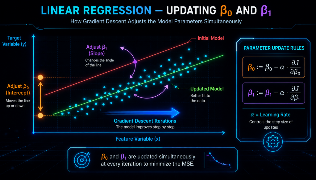
The intuition is that $β_{0}$ controls the height of the line: it shifts the whole thing up or down without changing its tilt. Picture a horizontal bar floating above your data; adjusting $β_{0}$ is raising or lowering it as a block until it sits centered among the points. That’s why it only cares about the average error, without paying attention to where the points sit along the x-axis.

3. Derivative with respect to β₁: the tilt adjustment

The derivative with respect to $β_{1}$ looks a lot like the previous one, but with one crucial detail:

$\partial β ^{1} \partial J = n 2 \sum_{i = 1 n} (y^_{i} - y_{i}) x_{i}$

See the difference? Each error shows up multiplied by its own $x_{i}$ . That tiny $x_{i}$ changes everything, because it makes the errors carry different weight depending on where they are.

The intuition is this: points that are far out on the x-axis (with a large $x_{i}$ ) have far more power to «rotate» the line. Think of a lever: the farther from the pivot you push, the more rotation you get with less force. The same thing happens here. An error at a distant point drags the slope far more strongly than the same error at a point near the origin.

That’s why we say $β_{1}$ controls the tilt of the line. While $β_{0}$ raises and lowers the whole line, $β_{1}$ rotates it so its angle follows the trend of the data.

4. The final update formulas

Now we put the two pieces together. Remember the Gradient Descent rule from Part 3: new value = current value − (learning rate) × (slope of the error). Substituting the derivatives we just computed, we get the two equations that are the real engine of training:

$β_{0} := β_{0} - α \cdot n 2 \sum_{i = 1 n} (y^_{i} - y_{i})$

$β_{1} := β_{1} - α \cdot n 2 \sum_{i = 1 n} (y^_{i} - y_{i}) x_{i}$

And here’s the important part, the one worth burning into your memory: this is all there is. Nothing more. These two subtractions, run together at every iteration, are literally what a linear regression model does to learn.

One detail that often slips by but is fundamental: both coefficients update at the same time, using the «old» values of $β_{0}$ and $β_{1}$ . You don’t update $β_{0}$ and then use that new value for $β_{1}$ . You compute both adjustments from the current line and then take both steps at once. It’s like adjusting the volume and the bass on a stereo: you move both based on how it sounds right now, you don’t chain one off the other.

5. Geometric intuition: adjusting a ruler on the table

If the formulas still feel abstract, this is probably the best mental image you can hold onto.

Imagine you have a table covered in points and a long ruler that you want to place so it passes as close as possible to all of them. What do you naturally do?

First you raise or lower it as a block, so it sits roughly at the height of the cloud of points. That’s adjusting $β_{0}$ .
Then you rotate it a little, so its tilt follows the trend of the data. That’s adjusting $β_{1}$ .
You check how it looks, see it’s still not perfect, and correct again the height and the angle.
You repeat over and over, with finer and finer adjustments, until the ruler sits in the most balanced position possible.

That’s exactly what the two formulas above do at each iteration: one pushes the line up or down, the other tilts it, and together they bring it closer to the data step by step. What for us is eye and hand, for the model is two subtractions.

6. A numerical example, step by step

Nothing clarifies more than watching the numbers actually move. Let’s run one full iteration with a single point, so we don’t get lost. (To make it easier to follow, we’ll simplify by leaving the scaling factor aside and working with a single data point; the logic is identical.)

We start from a model that kicks off with arbitrary values:

$β_{0} = 1$
$β_{1} = 2$
Learning rate: $α = 0.1$
Our point: $x = 3$ , $y = 10$

Step 1 — Predict with the current line:

$y^= 1 + 2 \cdot 3 = 7$

Step 2 — Measure the error. The real value was 10, but we predicted 7:

$y^- y = 7 - 10 = - 3$

The error is negative, which means we fell short: the line predicts below reality.

Step 3 — Update the coefficients:

$β_{0} := 1 - 0.1 \cdot (- 3) = 1 + 0.3 = 1.3$

$β_{1} := 2 - 0.1 \cdot (- 3) \cdot 3 = 2 + 0.9 = 2.9$

So what happened? The line went up ( $β_{0}$ moved from 1 to 1.3) and got steeper ( $β_{1}$ moved from 2 to 2.9). And it makes perfect sense: since we were predicting too low, the model reacts by lifting the line and increasing its slope to get closer to that point that had escaped above it.

If we now predicted again with the new coefficients, the error would be smaller. Repeat this thousands of times, across all your points, and you have a trained model.

7. When do we stop updating?

A logical question: if the model repeats these subtractions over and over, when does it decide it’s had enough? There are three common signals to stop, and they’re usually used in combination:

The error barely changes. If the improvement from one iteration to the next is tiny, carrying on is just wasting compute.
The gradient is nearly zero. Remember from Part 3 that the gradient flattens out as you approach the bottom of the valley. When it’s practically zero, it means we’re already at the lowest point and there’s nowhere left to descend.
A maximum number of iterations is reached. A safety limit we set ourselves so the process doesn’t run forever.

And here it’s worth recalling the great comfort of linear regression: because its error surface is convex (that bowl shape we saw in Part 2), we know we’ll always reach the same global minimum, no matter what values we started from. There’s no risk of getting stuck in a «false valley.» In more complex models, like neural networks, that’s no longer guaranteed, and that’s why knowing when to stop becomes something of an art there.

8. The same formula for Batch, SGD, and Mini‑batch

You might wonder how these formulas fit with the Gradient Descent variants we mentioned at the end of Part 3. The answer is beautiful in its simplicity: the formulas don’t change at all. The only thing that changes is how many errors you put inside that sum before updating.

Variant	How many points it uses in the sum
Batch GD	Sums the error over all the data before each update.
SGD	Sums the error of a single point and updates immediately.
Mini‑batch	Sums the error of a small batch (32, 64, 128…) and updates.

In other words, the example we did in section 6 with a single point is, technically, one step of SGD. If instead of one point we had averaged the error over the thousand points in the dataset, it would be Batch. And if we’d used a little group of 64, Mini‑batch. The update mechanism, the two subtractions, is always identical. That’s the elegant part: once you understand the formula, you understand all three variants at once.

In summary

$β_{0}$ and $β_{1}$ update using the derivatives of the MSE, which are nothing more than the average error (for $β_{0}$ ) and the error weighted by x (for $β_{1}$ ).
$β_{0}$ adjusts the height of the line; $β_{1}$ adjusts its tilt, and distant points have more power to rotate it.
The update formulas are two simple subtractions based on the gradient, applied simultaneously at each iteration.
Every step moves the line a little closer to the data, like someone adjusting a ruler on a table.
Thanks to convexity, we always reach the same global minimum.
And most importantly: this simple mechanism is the very foundation on which far more complex models learn, from logistic regression to neural networks.

Machine Learning, AI, Artificial Intelligence, General, IA, Inteligencia Artificial

| Tags: AI, artificial, ia, inteligencia, Inteligencia artificial, learning, machine, Machine Learning

De On-Premise a la Nube in English

How Linear Regression Learns: Coefficient Updates Explained (Part 4)