





Deep Learning: The Perceptron and the MLP
The birth of modern neural networks
How an idea as simple as «add up weights and fire a function» ended up creating all of Deep Learning.
So far we’ve toured the world of classic Machine Learning. PCA flattens universes, LDA draws boundaries, LSA uncovers meaning, t‑SNE reveals landscapes, and ensemble methods find strength in numbers. Each one, in its own way, is brilliant.
But all of them, however powerful, hit the same wall.
There are patterns you just can’t capture with trees, or regressions, or distances, or projections. Patterns too curved, too deep, too abstract for the tools we’ve seen. Think about recognizing a face in a photo, understanding the tone of a sentence, or predicting the next frame of a video: that’s where the classic methods throw up their hands and give up.
That’s exactly where Deep Learning is born.
And like every great story, it starts with something tiny. A minimal unit. An atom.
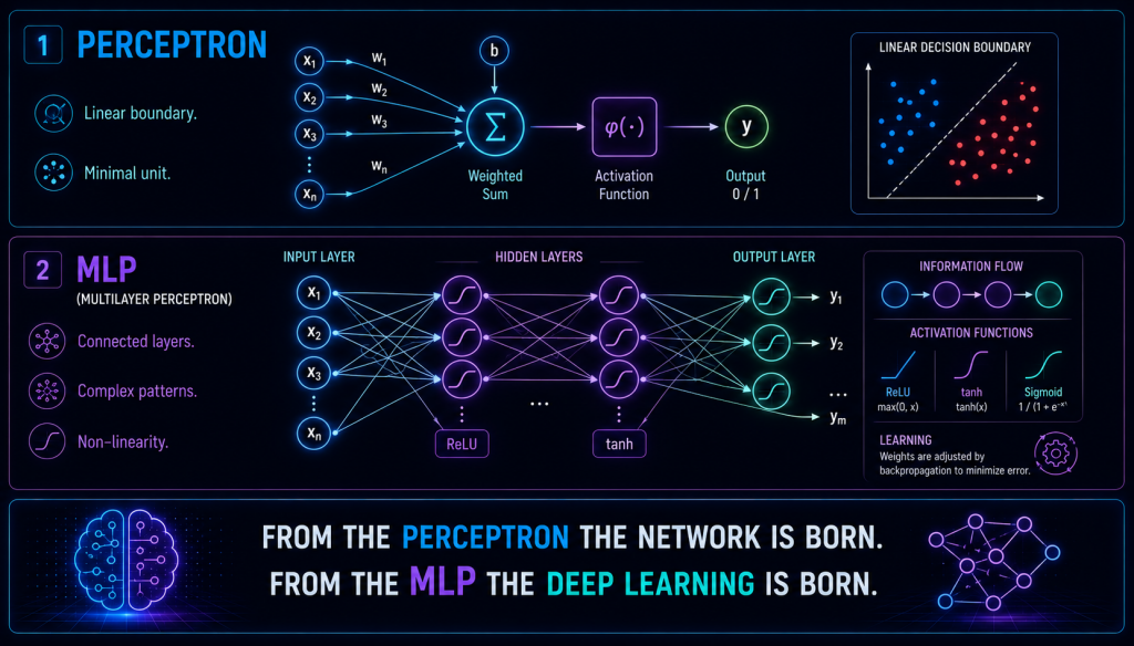
The perceptron.
The perceptron: the artificial neuron that started it all
The perceptron is the simplest idea you can have of a neuron. And how it works fits into four steps:
- It takes several inputs (the data).
- It multiplies each one by a weight (its importance).
- It adds everything up.
- It runs the result through a function that decides: yes or no?
It is, quite literally, a gate. A boundary. A straight line drawn across space.
Mathematically it’s almost trivial:
Where $f$ is usually a step function: if the sum crosses a certain threshold, the neuron «fires» and outputs a 1; if not, it stays at 0. The weights $w$ say how much each input matters, and $b$ (the bias) shifts the threshold one way or the other.
A silly example to make it click. Imagine you’re deciding whether to go for a run. Your inputs are: is it sunny? do you have time? do you feel like it? Each one carries a weight depending on how much it matters to you. You add them up, and if you clear your personal threshold… you lace up your shoes. That’s a perceptron.
It’s simple. It’s elegant. And it’s not enough.
The fatal limitation: the XOR problem
The perceptron has one huge Achilles’ heel: it can only learn linear boundaries. It only knows how to split the world with a straight line. And that means there are problems it will never solve, no matter how long you train it.
The classic example is XOR. The rule is simple: the answer is «yes» when the two inputs are different, and «no» when they’re the same. If you plot those four points on a plane, the «yes» points land in two opposite corners, and the «no» points in the other two. Crossed diagonally.
And there’s the drama: no straight line can separate them. No matter how you rotate, shift, or tilt it, it will always leave points from both classes mixed together.
The perceptron looks at that problem and can only say:
«Sorry, I can’t.»
That limitation weighed so heavily that, for years, much of the scientific community gave neural networks up for dead. Until someone asked a question that changed everything:
What if, instead of one perceptron, we connect many of them together?
The MLP: the first «real» neural network
An MLP (Multilayer Perceptron) is exactly that: a layer of perceptrons connected to another layer, connected to another, connected to another…
At its core, it’s a composition of functions. A chain of transformations. A machine that takes raw data and refines it step by step, layer by layer.
Its structure has three parts:
- Input layer → receives the data.
- Hidden layers → transform the information (this is where the magic happens).
- Output layer → produces the final prediction.
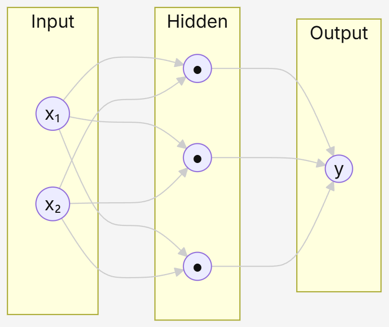
The key is that each layer applies a non-linear activation function (ReLU, tanh, sigmoid…). Those functions are what let the network bend, curve, and twist space instead of slicing it with a plain straight line.
And that’s where the miracle happens: connect two perceptrons, one behind the other, with a non-linearity in between… and XOR gets solved without breaking a sweat. What was impossible for a single neuron becomes trivial for a network.
With that power, an MLP learns:
- curved boundaries,
- complex patterns,
- non-linear combinations,
- deep relationships between variables.
It’s the first model that truly «thinks» in several steps.
The intuition: composing functions
Think of an MLP as an assembly line:
- The first layer detects simple patterns.
- The second combines those patterns into more complex structures.
- The third refines them even further.
- The last makes the decision.
It’s like learning to draw. First you sketch loose lines. Then shapes. Then shading. Then details. And in the end, almost without noticing, the full drawing appears.
An MLP does exactly that, but with math: it starts from the simple and builds up the complex, one level on top of another.
The problem: how do we tune all those weights?
Here comes the awkward question. A perceptron has a handful of parameters. An MLP can have thousands. A deep network, millions.
How do you adjust all of that? How does each neuron know what weight it should have? And when the network gets it wrong, how do you split the blame for the error across millions of parameters to figure out which one to fix, and by how much?
The answer is one of the most important algorithms in the history of Deep Learning:
Backpropagation.
But that’s the topic of the next chapter.
In summary
The perceptron is the minimal unit of Deep Learning: an artificial neuron that takes inputs, weighs them, and decides. But it’s trapped in straight lines: it can only learn linear boundaries.
The MLP is the revolution. A network of connected perceptrons that, thanks to activation functions and the composition of layers, learns patterns a single neuron could never capture.
It’s the first model that «thinks» in several steps. The first that can bend space. The first capable of solving what the perceptron deemed impossible.
And it’s the bridge to what comes next:
Backpropagation: the algorithm that teaches networks how to learn.